Sklearn Linear Regression on NFL Combine Data (Step by Step)
Sklearn linear regression takes three lines of Python. You create a LinearRegression() model, call .fit(X, y) on rows where you know the answer, and call .predict() on rows where you don’t. scikit-learn, which you import as sklearn, finds the straight line that fits your data best and hands you its slope and intercept.
In 12 steps, this tutorial predicts the 40-yard dash times of NFL Combine players. Weight alone explains about three quarters of the spread in their times. Add height and position, and on players it never saw, the model reaches an R-squared of 0.809, meaning it explains 80.9% of that spread. Then it replays two mistakes from my own class code, on purpose, so you can watch what they do to the score.
Every code block runs top to bottom on Python 3.14.7 with scikit-learn 1.9.1, pandas 3.1.1 and NumPy 2.5.4, and the output shown is what it printed. It ran in fresh virtual environments on Python 3.14.7 and 3.13.8 and printed the same output on both.
What is sklearn linear regression?
Linear regression predicts a number from one or more inputs. With one input it draws a line. With several, it fits a flat surface through all of them at once, which is called multiple linear regression.
scikit-learn is a free Python library for machine learning. The package is called scikit-learn, but you import it as sklearn, so both names lead to the same class, sklearn.linear_model.LinearRegression.
The LinearRegression docs call it “Ordinary least squares Linear Regression.” In plain words, it picks the line that makes the squared misses between its predictions and the real answers as small as possible.
After fit, the model holds two things you’ll read a lot.
coef_is the slope, one number per input. It says how much the prediction moves when that input goes up by one.intercept_is the prediction when every input is zero.
If you want p-values and confidence intervals for a single line, my SciPy linear regression tutorial covers scipy.stats.linregress. This post is the scikit-learn way, where the model plugs into train and test splits, pipelines and cross-validation.
What went wrong in my BDA 594 notebook?
My code for a group project in BDA 594, part of my Big Data Analytics master’s at SDSU, predicted how far NFL players move from their weight and their average speed. The data was NFL player tracking data our class was given. The notebook is public in my grad projects repo.
The README calls the model “a simple linear regression model created through an artificial neural network.” It was really a small Keras network, which I unpacked in the SciPy post. It had two problems, and neither one was the network’s fault.
The input already held the answer
The model predicted each player’s averageDistance2020 from weight and averageSpeed2020. Here are the first five players my notebook printed, with one column added.
| Average speed | Average distance | Speed divided by distance |
|---|---|---|
| 5.248913 | 0.526395 | 9.97 |
| 4.691877 | 0.470228 | 9.98 |
| 4.357956 | 0.436417 | 9.99 |
| 4.429058 | 0.444873 | 9.96 |
| 4.750842 | 0.475420 | 9.99 |
The ratio sits at almost exactly 10 for every player. The tracking timestamps in the same notebook are a tenth of a second apart, 18:03:02.200, then .300, then .400. So the numbers show that the distance column was distance per tenth of a second, which is just speed divided by 10.
The cell that made the distance column has a comment, “Average distance traveled per game, in yards.” The notebook’s own summary puts the average at 0.28 yards. That would be a very short game.
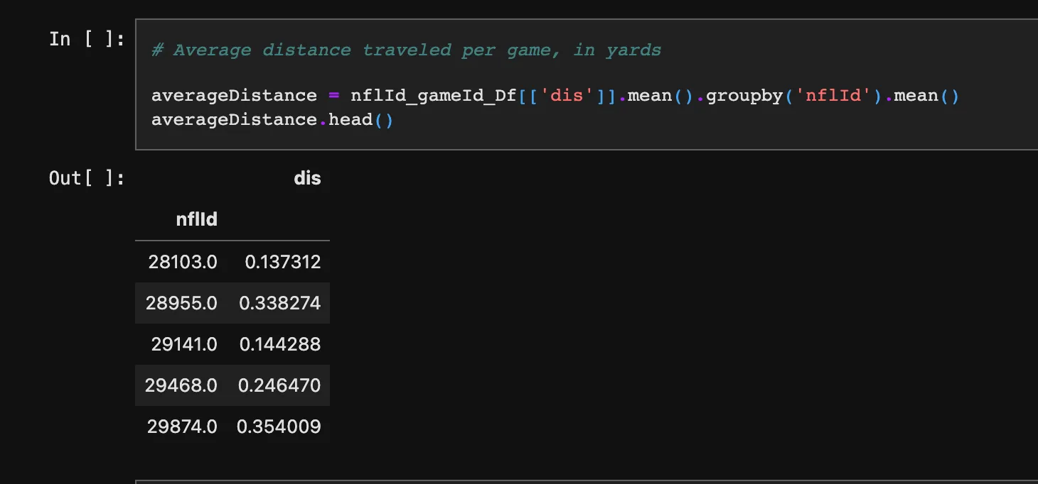
That cell in my class notebook on GitHub. Its rows are sorted by player ID, so they’re different players from the table above, which comes from a later cell after the merge. The comment says per game, but each value is an average over tracking frames a tenth of a second apart.
This is called data leakage. The scikit-learn docs on common pitfalls define it as “information that would not be available at prediction time is used when building the model.” The notebook’s goal was predicting new players. A new player with no tracking data has no average speed either, and once you have their tracking data you can compute the distance directly.
The scaler only touched the test set
I covered the second mistake in my Keras in Python tutorial. The code fit a MinMaxScaler on the training rows and scaled the test rows, but it never scaled the training rows. So the model trained on raw weights in pounds and was tested on squeezed ones.
The test weights even printed as -0.79. The cell that displays X_test shows -0.79140708 first, and all six rows it shows sit between -0.792 and -0.789. One pass of the scaler puts weights between about 0 and 1, and -0.79 is what you get when numbers that were already scaled go through it again, so the scaling cell most likely ran twice.
What did that do to the score?
My notebook printed a training loss of 0.0019 and a test loss of 0.0480, about 25 times worse on players it hadn’t trained on. That test loss is a mean squared error, so the root mean squared error was 0.219 yards.
The target’s standard deviation was 0.170 yards. A model that guesses the average for every player scores a root mean squared error about equal to the standard deviation, and Step 7 shows that happening on real data. So the input held the answer, and the model still lost to a guess.
Neither mistake needs a neural network. Both happen just as easily with plain linear regression, which is why Step 12 replays them.
What do you need before you start?
You need three things.
- Python 3.12 or newer. NumPy 2.5.4, which comes with pandas, requires it.
- A terminal and an internet connection, because pandas downloads the data straight from GitHub.
- Basic Python and a little pandas. If DataFrames are new to you, start with my pandas tutorial for beginners.
The 12 steps at a glance
Steps 1 to 7 give you a working model with a score you can trust. Steps 8 to 11 make it better and put it to work. Step 12 breaks it on purpose.
- Install scikit-learn and pandas in a virtual environment.
- Load the NFL Combine data from nflverse.
- Clean the rows and convert height to inches.
- Group the positions into eight groups.
- Hold out the 2026 class and split the rest.
- Fit a sklearn linear regression on weight.
- Score it against a guess.
- Add height and position with a pipeline.
- Cross-validate the model.
- Read the coefficients.
- Predict new players, including the whole 2026 class.
- Replay my two class mistakes on purpose.
Step 1. Install scikit-learn and pandas
Make a virtual environment first. That’s a private folder of packages for one project, so nothing here clashes with the rest of your Python setup. Any Python from 3.12 up works in place of python3.14.
python3.14 -m venv .venv
source .venv/bin/activate
pip install scikit-learn pandas
pip pulls in NumPy, SciPy and two small helpers along the way. These are the versions this tutorial ran on.
Python 3.14.7
joblib          1.6.0
numpy           2.5.4
pandas          3.1.1
python-dateutil 4.0.0
scikit-learn    1.9.1
scipy           1.18.1
threadpoolctl   3.7.0
tzdata          2026.6
Put the code from each step into one file, say combine.py, and run it with python combine.py. Or paste the steps into a Jupyter notebook one cell at a time.
Step 2. Load the NFL Combine data
The NFL Combine is a yearly event where college players are measured and timed before the NFL draft. nflverse publishes every Combine since 2000 as one CSV file. Its data is licensed under CC BY 4.0, which only asks you to give credit, and its release notes say the data is “courtesy of PFR,” short for Pro Football Reference.
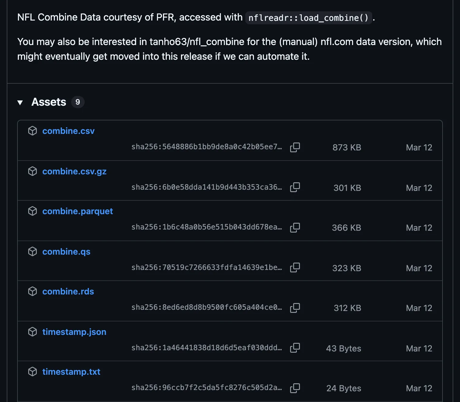
The combine release on GitHub. combine.csv is the file the code below loads.
pandas reads the file straight from the URL.
import pandas as pd

URL = "https://github.com/nflverse/nflverse-data/releases/download/combine/combine.csv"
combine = pd.read_csv(URL)

print(combine.shape)
print(combine[["season", "player_name", "pos", "ht", "wt", "forty"]].head())
(8968, 18)
season player_name pos ht wt forty
0 2000 John Abraham OLB 6-4 252.0 4.55
1 2000 Shaun Alexander RB 6-0 218.0 4.58
2 2000 Darnell Alford OT 6-4 334.0 5.56
3 2000 Kyle Allamon TE 6-2 253.0 4.97
4 2000 Rashard Anderson CB 6-2 206.0 4.55That’s 8,968 rows and 18 columns, one row per player per Combine. forty is the 40-yard dash in seconds, and it’s what the model will predict. wt is weight in pounds. ht is height as text, like 6-4 for six foot four, which is exactly how my class data stored it too.
The file nflverse serves was last updated on March 12, 2026, and every run here pulled it on November 4, 2026. If nflverse updates it, your counts will differ a little.
Step 3. Clean the rows and convert height to inches
First, count the blanks in the three columns the model needs.
print(combine[["ht", "wt", "forty"]].isna().sum())ht 29
wt 24
forty 929
dtype: int64929 players have no 40 time, and a few have no height or weight. A model can’t learn from a blank, so those rows go.
players = combine.dropna(subset=["ht", "wt", "forty"]).copy()

feet_inches = players["ht"].str.split("-", expand=True).astype(int)
players["height_in"] = feet_inches[0] * 12 + feet_inches[1]

players = players[~players["pos"].isin(["K", "P", "LS"])]
print(len(players), "players left")
print(players["forty"].agg(["min", "mean", "max"]).round(2))
7826 players left
min 4.21
mean 4.76
max 6.05
Name: forty, dtype: float64str.split("-", expand=True) splits 6-4 into two columns, 6 and 4. Feet times 12 plus inches gives height in inches, a number the model can use.
The last filter drops kickers, punters and long snappers, the special teams specialists. My class notebook dropped punters and kickers the same way. They’re a small group that doesn’t fit the position groups in the next step.
That leaves 7,826 players, with 40 times from 4.21 to 6.05 seconds.
Step 4. Group the positions
The Combine’s position labels changed over the years. Guards are OG up to 2023 and G from 2024. Safeties are S up to 2022 and SAF from 2024. ILB stops in 2018, the year plain LB and EDGE first appear. A dictionary maps all 21 labels to eight groups.
GROUPS = {
    "QB": "QB", "RB": "RB", "FB": "RB", "WR": "WR", "TE": "TE",
    "C": "OL", "G": "OL", "OG": "OL", "OT": "OL", "OL": "OL",
    "DE": "DL", "DT": "DL", "DL": "DL", "EDGE": "DL",
    "ILB": "LB", "OLB": "LB", "LB": "LB",
    "CB": "DB", "S": "DB", "SAF": "DB", "DB": "DB",
}
players["group"] = players["pos"].map(GROUPS)

print(players["group"].isna().sum(), "players without a group")
print(players.groupby("group")["forty"].agg(["count", "mean"]).round(2).sort_values("mean"))
0 players without a group
count mean
group
WR 1159 4.51
DB 1479 4.52
RB 835 4.58
LB 865 4.69
TE 452 4.76
QB 413 4.81
DL 1288 4.93
OL 1335 5.24map swaps each label for its group, and the first line confirms that no label was left out. Fullbacks go with running backs, and EDGE goes with the defensive line.
The averages already tell a story. Wide receivers and defensive backs run about 4.5 seconds, and offensive linemen run 5.24. Keep that gap in mind for Step 8.
Step 5. Hold out the 2026 class and split the rest
A model has to be judged on players it never studied, so this step sets aside two kinds of unseen data.
First, the whole 2026 class goes in a drawer until Step 11. That’s the closest thing to predicting a real new class.
history = players[players["season"] < 2026]
new_class = players[players["season"] == 2026]

print(len(history), "players from 2000 to 2025")
print(len(new_class), "players from the 2026 combine")
7637 players from 2000 to 2025
189 players from the 2026 combineThen train_test_split shuffles the other 7,637 players and keeps 20% back as a test set. The model learns from the training rows only. The test rows are the exam, and random_state=42 makes the shuffle the same every time you run it.
from sklearn.model_selection import train_test_split

train, test = train_test_split(history, test_size=0.2, random_state=42)
print(len(train), "training rows,", len(test), "test rows")
6109 training rows, 1528 test rowsA model that does well in training and badly on the test set has memorized instead of learned. My post on overfitting vs underfitting shows how to tell the two apart.
Step 6. Fit a sklearn linear regression on weight
Start with one input, weight.
from sklearn.linear_model import LinearRegression

model = LinearRegression()
model.fit(train[["wt"]], train["forty"])

print(f"slope     {model.coef_[0]:.5f} seconds per pound")
print(f"intercept {model.intercept_:.3f} seconds")
slope 0.00581 seconds per pound
intercept 3.351 secondstrain[["wt"]] has double brackets on purpose. scikit-learn wants the inputs as a table, one row per player and one column per input, even when there’s only one input. Single brackets give you a single column instead, and fit stops with ValueError: Expected a 2-dimensional container but got <class 'pandas.Series'> instead.
The slope is 0.00581 seconds per pound, so every extra 10 pounds adds about 0.058 seconds to the 40. The intercept, 3.351 seconds, is the predicted time for a player who weighs nothing. That’s why nobody reads an intercept on its own.
Now predict four sizes of player.
sizes = pd.DataFrame({"wt": [190, 220, 250, 310]})
print(sizes.assign(forty=model.predict(sizes).round(2)))
wt forty
0 190 4.45
1 220 4.63
2 250 4.80
3 310 5.15predict takes a table with the same column name the model trained on. Here’s the line against the players from 2000 to 2025, grouped into 10-pound bands.
Rendered with Python from the run's output.
Step 7. Score it against a guess
A prediction is only useful if you know how far off it tends to be. scikit-learn has a function for each of the three scores you’ll see most.
- R-squared, the share of the spread in 40 times the model explains. 1 is perfect. 0 is no better than guessing the average.
- MAE, mean absolute error, the average miss in seconds.
- RMSE, root mean squared error, also in seconds. Squaring before averaging makes big misses count more.
A small helper prints all three for any model, so the rest of the post can reuse it.
from sklearn.metrics import mean_absolute_error, r2_score, root_mean_squared_error


def report(name, actual, predicted):
    r2 = r2_score(actual, predicted)
    mae = mean_absolute_error(actual, predicted)
    rmse = root_mean_squared_error(actual, predicted)
    print(f"{name:<17} R2 {r2:6.3f}  MAE {mae:.3f} s  RMSE {rmse:.3f} s")


report("weight only", test["forty"], model.predict(test[["wt"]]))
print("model.score:", round(model.score(test[["wt"]], test["forty"]), 3))
weight only R2 0.747 MAE 0.117 s RMSE 0.153 s
model.score: 0.747On 1,528 players it never trained on, the weight-only line misses by 0.117 seconds on average and explains 74.7% of the spread.
The last line asks the model itself. LinearRegression has a score method, and the LinearRegression docs say it will “Return coefficient of determination on test data.” That’s R-squared’s full name, so model.score and r2_score print the same 0.747.
Is that good? Compare it with a model that ignores weight completely. DummyRegressor learns the average 40 time from the training rows and predicts it for everyone.
from sklearn.dummy import DummyRegressor

guess = DummyRegressor(strategy="mean")
guess.fit(train[["wt"]], train["forty"])

report("guess the average", test["forty"], guess.predict(test[["wt"]]))
print(f"standard deviation of the test set {test['forty'].std(ddof=0):.3f} s")
guess the average R2 -0.000 MAE 0.251 s RMSE 0.304 s
standard deviation of the test set 0.304 sGuessing the average scores an R-squared of zero, by definition. The minus sign is rounding, because the training average sits a hair away from the test average. Its RMSE, 0.304, matches the test set’s standard deviation. My class notebook printed its RMSE and its standard deviation a few cells apart and never put them side by side.
So one input halves the RMSE of a pure guess, from 0.304 to 0.153 seconds. Always score a guess first. It takes three lines and tells you whether your model learned anything at all.
Step 8. Add height and position with a pipeline
Adding an input is the same call with one more column.
both = LinearRegression()
both.fit(train[["wt", "height_in"]], train["forty"])

report("weight + height", test["forty"], both.predict(test[["wt", "height_in"]]))
print("coefficients", both.coef_.round(5))
print(f"height alone vs forty, correlation {train['height_in'].corr(train['forty']):.2f}")
print(f"height vs weight, correlation {train['height_in'].corr(train['wt']):.2f}")
weight + height R2 0.748 MAE 0.117 s RMSE 0.152 s
coefficients [ 0.006 -0.00461]
height alone vs forty, correlation 0.60
height vs weight, correlation 0.72Height barely moves the score, from 0.747 to 0.748. On its own, height tracks the 40 time closely, with a correlation of 0.60. But tall players also tend to be heavier, with a correlation of 0.72 between the two, and once weight is in the model, height has almost nothing left to add. Height looked guilty until weight walked in.
Position is a different story, but it’s text, and LinearRegression only takes numbers. Three scikit-learn tools get the columns ready.
OneHotEncoderturns thegroupcolumn into one column per group, holding 1 for the player’s group and 0 for the rest.drop="first"leaves out the first group alphabetically, DB, so every other group is measured against defensive backs.StandardScalerrescales weight and height so each has an average of 0 and a standard deviation of 1.ColumnTransformerapplies each one to its own columns.
Then make_pipeline chains that preparation and the model into one object, called a pipeline. When you call fit, it learns the scaling from the training rows only. When you call predict, it applies that same scaling to whatever rows you pass in.
make_pipeline wraps all of it, so fit learns the scaling, the groups and the coefficients from the training rows only.from sklearn.compose import ColumnTransformer
from sklearn.pipeline import make_pipeline
from sklearn.preprocessing import OneHotEncoder, StandardScaler
FEATURES = ["wt", "height_in", "group"]
prep = ColumnTransformer([
("numbers", StandardScaler(), ["wt", "height_in"]),
("position", OneHotEncoder(drop="first"), ["group"]),
])
pipe = make_pipeline(prep, LinearRegression())
pipe.fit(train[FEATURES], train["forty"])
report("+ position group", test["forty"], pipe.predict(test[FEATURES]))+ position group R2 0.809 MAE 0.103 s RMSE 0.133 sPosition lifts R-squared from 0.748 to 0.809, and the average miss drops to 0.103 seconds. The common pitfalls page puts the main benefit plainly. “The scikit-learn pipeline is a great way to prevent data leakage as it ensures that the appropriate method is performed on the correct data subset.”
Where does the weight-only line miss?
A residual is one miss, the real time minus the predicted time. A positive residual means the player ran slower than predicted. If a model fits well, its residuals average out near zero in every slice of the data. Group them by weight and you can see what position fixed. The last line, pd.crosstab, counts the test players in each band by position group.
misses = pd.DataFrame({
    "weight only": test["forty"] - model.predict(test[["wt"]]),
    "with position": test["forty"] - pipe.predict(test[FEATURES]),
})
bands = pd.cut(test["wt"], [0, 200, 240, 280, 320, 400],
               labels=["under 200", "200-240", "240-280", "280-320", "over 320"])
table = misses.groupby(bands, observed=True).mean().round(3)
table["players"] = bands.value_counts()
print(table)
print(pd.crosstab(bands, test["group"]))
weight only with position players
wt
under 200 0.038 0.017 306
200-240 0.001 -0.001 518
240-280 -0.071 -0.015 316
280-320 0.025 0.001 316
over 320 0.061 0.035 72
group DB DL LB OL QB RB TE WR
wt
under 200 163 0 0 0 3 25 0 115
200-240 118 1 73 0 81 127 4 114
240-280 0 117 76 1 4 19 97 2
280-320 0 118 1 197 0 0 0 0
over 320 0 13 0 59 0 0 0 0The weight-only line has a pattern. Players from 240 to 280 pounds ran 0.071 seconds faster than it predicted. Of the 316 in that band, 290 are defensive linemen, linebackers or tight ends, heavy players who are built to run. Players over 320 pounds ran 0.061 seconds slower, and 59 of those 72 are offensive linemen.
With position in the model, four of the five bands land within 0.017 seconds of zero. The heaviest players still run 0.035 seconds slower than predicted, because a straight line can’t bend at the end. The FAQ at the bottom covers a model that can.
One thing worth knowing. Plain linear regression doesn’t need scaling at all. The same pipeline without the scaler makes the same predictions.
import numpy as np

plain = make_pipeline(
    ColumnTransformer([
        ("numbers", "passthrough", ["wt", "height_in"]),
        ("position", OneHotEncoder(drop="first"), ["group"]),
    ]),
    LinearRegression(),
)
plain.fit(train[FEATURES], train["forty"])

print("same predictions:", np.allclose(plain.predict(test[FEATURES]), pipe.predict(test[FEATURES])))
same predictions: TrueSo why keep the scaler? It changes what the coefficients mean, which Step 10 uses. And if you later swap in a model that does care about scale, like Ridge regression or a neural network, the pipeline already handles it.
Step 9. Cross-validate the model
One test set is one roll of the dice. Cross-validation rolls five times. KFold cuts the data into five parts, trains on four and tests on the fifth, then rotates until every player has been tested once.
from sklearn.model_selection import KFold, cross_val_score

folds = KFold(n_splits=5, shuffle=True, random_state=42)
scores = cross_val_score(pipe, history[FEATURES], history["forty"], cv=folds, scoring="r2")

print(scores.round(3))
print(f"mean {scores.mean():.3f}, spread {scores.std():.3f}")
[0.809 0.803 0.802 0.809 0.809]
mean 0.806, spread 0.003shuffle=True matters here, because the CSV is sorted by season. Without it, each part would be a block of years. cross_val_score fits a fresh copy of the pipeline for every split, so the scaler never learns from the part being tested.
All five scores land between 0.802 and 0.809. The 0.809 from Step 8 wasn’t a lucky split. The scikit-learn guide on cross-validation covers the other ways to split, like by group or by time.
Step 10. Read the coefficients
The fitted pipeline remembers every number it learned. get_feature_names_out gives you a name for each coefficient.
names = pipe[:-1].get_feature_names_out()
print(pd.Series(pipe[-1].coef_, index=names).round(3))
print(f"intercept {pipe[-1].intercept_:.3f}")
print("one standard deviation", pipe[0].named_transformers_["numbers"].scale_.round(1))
numbers__wt 0.229
numbers__height_in -0.035
position__group_DL 0.037
position__group_LB -0.005
position__group_OL 0.225
position__group_QB 0.209
position__group_RB -0.049
position__group_TE 0.033
position__group_WR -0.011
dtype: float64
intercept 4.717
one standard deviation [45.9 2.7]Each coefficient is the change in the predicted 40 time when its input goes up by one unit and every other input stays the same. Because of the scaler, one unit of weight or height is one standard deviation, which the last line prints, 45.9 pounds and 2.7 inches.
- Weight, 0.229. Every 45.9 extra pounds adds 0.229 seconds, at the same height and position.
- Height, -0.035. At the same weight and position, 2.7 more inches takes 0.035 seconds off. Tall and light beats short and heavy.
- Position groups, each compared with defensive backs of the same size. Offensive linemen run 0.225 seconds slower and quarterbacks 0.209 slower. Running backs run 0.049 faster. Linebackers and wide receivers are within about a hundredth of a second.
- Intercept, 4.717. With the scaler, this is the predicted time for a defensive back of average weight and height.
A coefficient is an average effect across thousands of players. The figure in Step 6 shows how widely real players spread around it.
Step 11. Predict new players
Pass the pipeline a table with the same column names it trained on. It scales and encodes the new row for you.
rookie = pd.DataFrame({"wt": [220], "height_in": [73], "group": ["WR"]})
print(f"{pipe.predict(rookie)[0]:.2f} seconds")
4.60 secondsA 220-pound, six-foot-one wide receiver gets 4.60 seconds. My class notebook also predicted a made-up 220-pound player.
Now the real test. Refit the pipeline on all 7,637 players from 2000 to 2025, then score the 2026 class it has never seen.
pipe.fit(history[FEATURES], history["forty"])
new_pred = pipe.predict(new_class[FEATURES])

report("2026 class", new_class["forty"], new_pred)

table = new_class.assign(predicted=new_pred.round(2))
table = table[["player_name", "group", "wt", "forty", "predicted"]].sort_values("forty")
print(table.head(3))
print(table.tail(3))
2026 class R2 0.753 MAE 0.114 s RMSE 0.142 s
player_name group wt forty predicted
8938 Brenen Thompson WR 164.0 4.26 4.37
8800 Lorenzo Styles Jr. DB 194.0 4.27 4.48
8937 Zavion Thomas WR 190.0 4.28 4.49
player_name group wt forty predicted
8921 Beau Stephens OL 315.0 5.35 5.24
8669 Markel Bell OL 346.0 5.36 5.36
8721 Garrett DiGiorgio OL 319.0 5.36 5.25On a brand new class, the model misses by 0.114 seconds on average, a little worse than its test score in Step 8. Look at the edges, though. The three fastest players in the class all ran faster than predicted, by 0.11 to 0.21 seconds, and two of the three slowest ran 0.11 seconds slower. Six players aren’t a pattern on their own, so group the residuals like Step 8 before you trust the model at either end.
Step 12. Replay my two class mistakes on purpose
Both mistakes from my BDA 594 notebook fit in a few lines of scikit-learn. These are deliberate replays, so don’t copy them into real code.
Replay 1. Hand the model the answer
My class mistake gave the model distance per tenth of a second as the target and speed as an input. Here’s the same shape. Speed in yards per second is 40 divided by the 40 time, the very number we’re predicting.
leaky = history.assign(yards_per_sec=40 / history["forty"])
leak_train, leak_test = train_test_split(leaky, test_size=0.2, random_state=42)

cols = ["wt", "yards_per_sec"]
cheat = LinearRegression()
cheat.fit(leak_train[cols], leak_train["forty"])

report("leak replay", leak_test["forty"], cheat.predict(leak_test[cols]))
leak replay R2 0.996 MAE 0.016 s RMSE 0.020 sAn R-squared of 0.996 on real people isn’t a breakthrough. It’s a confession. The model didn’t learn anything about football. It learned to undo a division.
To catch it, ask one question about every input. Would I have this number for a new player before I know the answer? If not, it’s leaking. And treat a near-perfect score on messy real data as a reason to look, not to celebrate.
Replay 2. Scale only the test set
This is the line my notebook had, without the line it was missing.
from sklearn.preprocessing import MinMaxScaler

X_train = train[["wt"]].to_numpy()
X_test = test[["wt"]].to_numpy()

scaler = MinMaxScaler()
scaler.fit(X_train)
X_test = scaler.transform(X_test)        # my notebook had this line
# X_train = scaler.transform(X_train)    # and was missing this one

broken = LinearRegression()
broken.fit(X_train, train["forty"])
broken_pred = broken.predict(X_test)

report("scaler replay", test["forty"], broken_pred)
print("first three predictions", broken_pred[:3].round(2))
scaler replay R2 -21.613 MAE 1.411 s RMSE 1.443 s
first three predictions [3.35 3.35 3.35]The model learned its slope on weights in pounds, then got test weights squeezed between 0 and 1. Every prediction lands at about the intercept, 3.35 seconds, for every player. The fastest 40 in the whole dataset is 4.21.
An R-squared of -21.613 means its squared misses add up to about 22.6 times those of guessing the average. The docs’ rule is short. “The general rule is to never call fit on the test data.” My bug was the mirror image, scaling the test rows and forgetting the training rows. The pipeline in Step 8 prevents both, because scaling lives inside the model and runs on whatever rows you pass.
Here’s every model in this post on the same test players.
Rendered with Python from the run's output.
The same models with all three scores, plus the cross-validation and the 2026 class.
| Model | Scored on | R-squared | MAE | RMSE | Step |
|---|---|---|---|---|---|
| Guess the average | 1,528 test players | -0.000 | 0.251 s | 0.304 s | 7 |
| Weight only | 1,528 test players | 0.747 | 0.117 s | 0.153 s | 7 |
| Weight and height | 1,528 test players | 0.748 | 0.117 s | 0.152 s | 8 |
| Weight, height and position | 1,528 test players | 0.809 | 0.103 s | 0.133 s | 8 |
| Same pipeline, five folds | 7,637 players | 0.806 average | Not printed | Not printed | 9 |
| Same pipeline, refit on 2000 to 2025 | 189 players from 2026 | 0.753 | 0.114 s | 0.142 s | 11 |
| Leak replay | 1,528 test players | 0.996 | 0.016 s | 0.020 s | 12 |
| Scaler replay | 1,528 test players | -21.613 | 1.411 s | 1.443 s | 12 |
When is linear regression the wrong tool?
- The answer is a category. Linear regression predicts a number, like a time in seconds. For yes or no, or for one of several classes, you need a classifier. My post on supervised vs unsupervised learning explains regression and classification side by side.
- The data curves. If the residuals show a pattern, like the weight-only line in Step 8, a straight line is missing the shape. The FAQ below shows the fix.
- Your inputs move together and you want to read the coefficients. Height and weight have a correlation of 0.72 in Step 8. The scikit-learn guide to linear models warns that when features are correlated, “the least-squares estimate becomes highly sensitive to random errors in the observed target.” It describes Ridge regression as a fix that works “by imposing a penalty on the size of the coefficients.”
- You need answers far outside your data. The training players weighed 149 to 375 pounds. The intercept in Step 6, 3.351 seconds for a player who weighs nothing, shows what a line does where it has no data.
What else do people ask about sklearn linear regression?
Does sklearn linear regression give p-values?
No. LinearRegression gives you coefficients, an intercept and the score method, and its docs never mention p-values. The OLS model in statsmodels does. Install it with pip install statsmodels, which gave version 0.15.0 here, and fit the weight and height model from Step 8 on the same training rows.
import statsmodels.api as sm

ols = sm.OLS(train["forty"], sm.add_constant(train[["wt", "height_in"]])).fit()
print(ols.summary().tables[1])
==============================================================================
coef std err t P>|t| [0.025 0.975]
------------------------------------------------------------------------------
const 3.6439 0.067 54.311 0.000 3.512 3.775
wt 0.0060 6.06e-05 99.070 0.000 0.006 0.006
height_in -0.0046 0.001 -4.425 0.000 -0.007 -0.003
==============================================================================The coefficients match what LinearRegression found in Step 8, 0.006 for weight and -0.0046 for height. P>|t| is the p-value, and the last two columns are a 95% confidence interval for each coefficient. All three p-values round to 0.000, so if a true coefficient were zero, you’d almost never see one this far from zero by chance.
Height’s p-value is tiny even though height barely moved R-squared in Step 8. With 6,109 training players, even a small effect is easy to tell apart from zero. A small p-value says an effect is there, not that it’s big.
For a single input, my SciPy linear regression tutorial gets the p-value from linregress and puts a confidence interval on the slope.
Is multiple linear regression a different class in sklearn?
No. It’s the same LinearRegression. You pass more columns, and it fits one coefficient per column, which is what Step 8 does with weight, height and position.
Can sklearn linear regression fit a curve?
Yes, with one extra step. PolynomialFeatures adds columns like weight squared, and LinearRegression fits a line through those columns, which draws a curve through the original data. The scikit-learn guide says the result is “still a linear model,” because it’s linear in its coefficients. Put both in a pipeline, the way Step 8 does with the scaler. This post didn’t fit one, so treat it as a next experiment for the heaviest players.
What should you remember about sklearn linear regression?
LinearRegression().fit(X, y)and then.predict(X_new). X is a table, so use double brackets for a single column.- Score on a test set the model never saw, and compare with
DummyRegressor. If you can’t beat the average, stop and look. - R-squared is the share explained, MAE is the typical miss in real units, and RMSE weighs big misses more.
- Group the residuals. A pattern means the line is missing the shape of the data.
- Put scaling and encoding in a pipeline with a
ColumnTransformer, sofitonly ever learns from training rows. - Plain linear regression doesn’t need scaling. Scaling changes how you read the coefficients.
- Cross-validate before you trust one split.
- A near-perfect score on real data is a warning sign. Check every input for the answer in disguise.
What’s the most suspicious R-squared you’ve ever been proud of?