Einstein 3, Me 0 (My Impulsive Attempt at General Relativity in Python)
A few months ago I drafted a research plan with Claude to rebuild space navigation on Einstein instead of Newton. It had a name, a NASA target and an 18-month roadmap. I never built any of it. This week I finally ran general relativity in Python against three of the plan’s own tests.
One thing up front. I’m a software developer, not a physicist or an astrophysicist, and in this field I’m probably a noob. Actually, scratch the “probably.” I did this for the love of the game, because my passion for deep space pulled me into this weird experiment.
My background is data. I have a master’s in Big Data Analytics from San Diego State, I work in data analytics at San Diego Unified School District, and I’ve built machine learning models for crypto price forecasting and NFL special teams. I even co-wrote a bioinformatics paper in 2019.
None of that taught me general relativity. It did make Python, NumPy and SciPy feel like home, and it gave me two habits this experiment needed, reading research papers and checking every model against real measurements.
So I didn’t try to judge the physics. I checked whether the code’s numbers match what people have actually measured, and where I’m leaning on a source instead, I say so. Read this as a curious data person’s notebook, not a physics paper.
Quick background. Newton treats gravity as a pull between two masses [1]. Einstein says mass bends space and time, and objects simply follow the bends [2]. My plan claimed spacecraft navigation was stuck on Newton’s version and needed rebuilding on Einstein’s. I hoped it could help us reach other stars.
The tests worked. Three short Python scripts, using SciPy and Astropy, reproduced three famous results that Newton gets wrong, from Mercury’s orbit, starlight passing the Sun, and GPS satellite clocks. But they also exposed the catch. Einstein’s version turned out to be Newton’s equation plus one small extra term, and NASA JPL’s planet tables already include it [3]. So GSNF can’t give spacecraft better routes, and it can’t get us to other stars.
I also rebuilt the plan’s most extreme case, an orbit right next to a black hole, as a 3D simulation you can spin around in your browser. I built it with Claude Code, and the prompt is at the end if you want to try it.
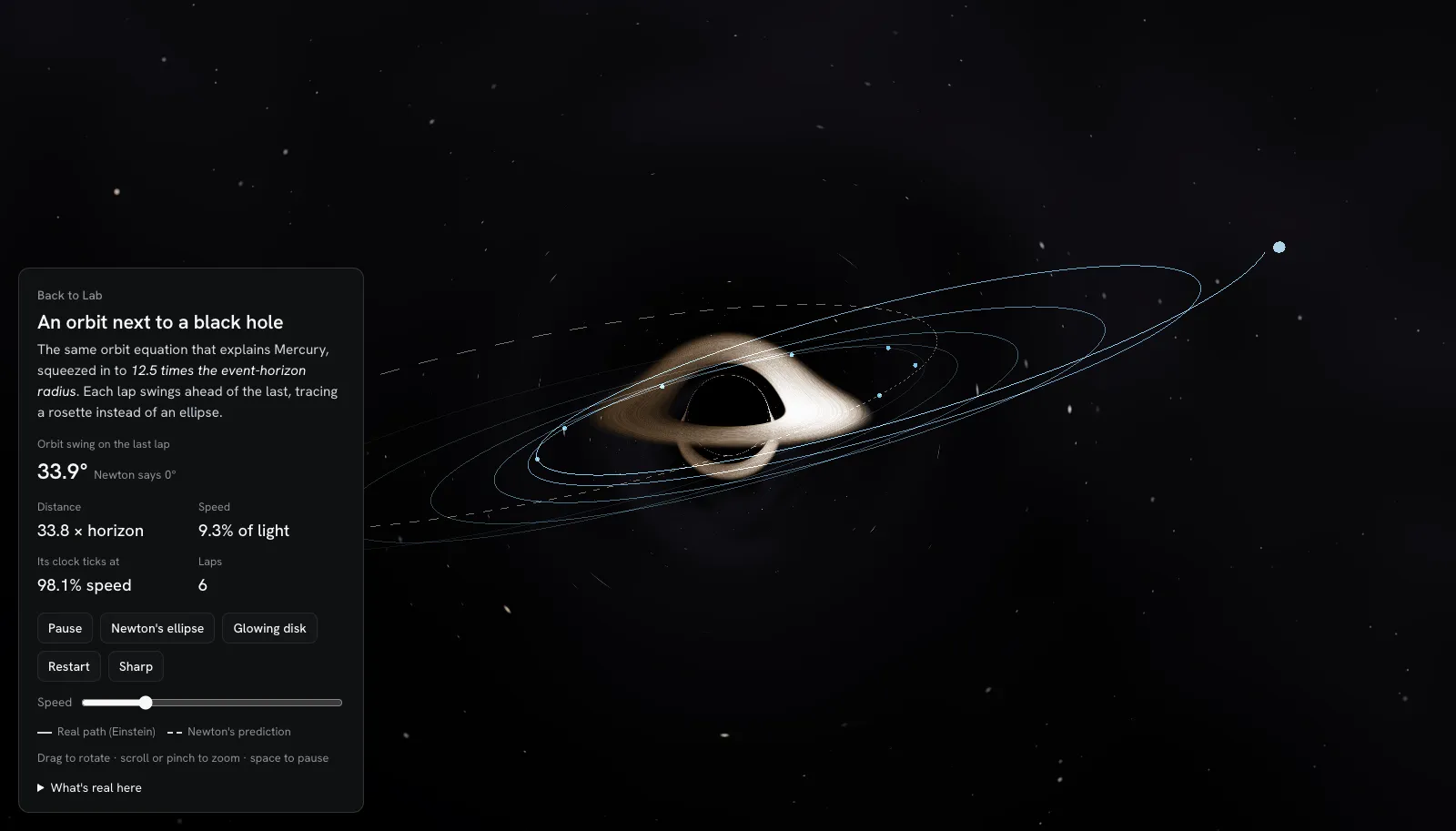
The 3D simulation after six laps. Each lap swings 33.9 degrees ahead of the last, where Newton’s gravity says 0.
What was my plan to rebuild space navigation?
I wrote it in May 2026 while I was thinking a lot about interstellar travel, gravity and relativity. I love deep space theories, and I’ve watched Interstellar probably a few times. So I sat down with Claude and drafted something that read like a grant proposal.
I called it the Geometric Spacetime Navigation Framework, or GSNF. Its founding rule sounded airtight.
If a principle cannot be cited, confirmed, and demonstrated through published and tested physics, it does not enter the framework.
The premise was bolder. It claimed that space exploration is “architecturally built on Newtonian force-based intuition, with relativistic corrections added as patches on top.” The fix was to start from Einstein’s picture, where gravity isn’t a force at all. Mass curves spacetime, the single fabric that space and time form together, and objects coast along the straightest possible paths through that curve. Physicists call those paths geodesics.
Think of a flight from New York to Tokyo. On a flat map it looks like a curve up over Alaska, but on the globe it’s the straightest route there is. A geodesic is the same idea in curved spacetime. Here’s what that looks like for light passing a black hole.
Rendered with Python and Manim.
On top of that sat a quantum layer about time emerging from entanglement. Then came ten Python libraries, three phases over 18 months, and a goal of a framework “compelling enough to present to NASA’s Innovative Advanced Concepts (NIAC) program within 18 months.” NIAC is real. It funds early ideas that could change future NASA missions.
There was even a companion document, a learning path promising that a focused software engineer could build the foundation in “three to four months of consistent part-time study.”
Between my lack of time and my lack of field experience, both stayed documents. Nothing in them ever ran. This post is the first time the tests have.
How was GSNF supposed to help space travel?
Two things were in my head, reaching other stars and finding better routes through deep space. The plan turned that into four promises.
- Better routes. Phase 2 reframed trajectory planning from “overcoming gravitational force” to “finding optimal geodesics through spacetime geometry.”
- Better clocks. It promised tools for “time synchronization” that were correct “from the first line of code.”
- A bigger payoff the farther out you go. Its closing said space travel built on Einstein would pull away from space travel built on Newton, and “the divergence grows larger the deeper into extreme gravitational environments we go.”
- A path to other stars. Phase 3 would study the Alcubierre warp drive, a real solution to Einstein’s equations where space shrinks in front of a ship and stretches behind it. The plan also cited a classic paper called “Wormholes in Spacetime and Their Use for Interstellar Travel.”
On paper, it read like a ticket to the stars.
How do you test general relativity in Python?
The best idea in the plan was its validation rule. Before any new physics, the code had to reproduce effects that were measured long ago. They’re tiny. An arcsecond is 1/3600 of a degree, about the width of a US quarter seen from 5 kilometers away. But they’re measured so precisely that any mistake in the code shows up right away.
Here’s how my three scripts did. The Newton column is what Newton’s gravity alone predicts.
| Test | Newton | Einstein (my code) | Real world | Source |
|---|---|---|---|---|
| Mercury’s extra orbit drift, arcseconds per century | 0 | 42.98 | 43 | [4] |
| Starlight bending at the Sun’s edge, arcseconds | 0.876 | 1.751 | 1.75 | [4] |
| GPS satellite clock vs a ground clock, microseconds per day | 0 | +38.4 | about +38 | [5] |
Numbers in brackets point to the references at the end, so you can check every figure yourself.
You don’t need the heavy relativity libraries the plan listed for any of this. Karl Schwarzschild solved Einstein’s equations for one round object that isn’t spinning, and the Sun spins slowly enough to count [6]. Sean Carroll’s lecture notes on general relativity walk from that solution to a single equation for a planet’s orbit. The derivation lives in his notes. My code only uses the result, which tracks u, 1 divided by the planet’s distance from the Sun, as the planet goes around.
Newton:    u'' + u = GM/h²
Einstein:  u'' + u = GM/h² + 3GM·u²/c²
Only the last term is new. That’s the whole difference between Newton and Einstein here, and Carroll’s notes make the same point [6]. For the rest, G is the gravitational constant, M is the Sun’s mass, c is the speed of light, and h measures how fast the planet sweeps sideways around the Sun. Read u’’ as how sharply u bends as the angle grows. You never solve this by hand, because SciPy steps through it in tiny slices.
Mercury’s perihelion in about 40 lines of Python
The perihelion is the point where Mercury swings closest to the Sun. Under Newton, with just the Sun and Mercury, the planet comes back to the exact same perihelion every lap. Under Einstein, it lands a little further around each time. Astronomers call that drift perihelion precession.
The script below uses SciPy’s solve_ivp, a solver that steps an equation forward in tiny slices, to run one lap under each equation. Its events option flags the moment u stops growing, which is the next closest approach, and the script measures how far past a full circle that lands. DOP853 picks one of SciPy’s high-accuracy solvers.
Mercury’s orbit comes from the NASA Mercury fact sheet, and the Sun’s constants come from Astropy, which uses the official values set by the International Astronomical Union in 2015. The script divides distances by the orbit’s size so the numbers stay near 1. Otherwise u would sit around 0.00000000002, and SciPy’s error limit for tiny values, atol, would be far too loose to mean anything.
import numpy as np
from scipy.integrate import solve_ivp
from astropy import constants as const

GM = const.GM_sun.value      # the Sun's G times M, in m^3/s^2
c = const.c.value            # speed of light, m/s

# Mercury's orbit (NASA Mercury fact sheet)
a = 57.909e9                 # semi-major axis, m
e = 0.2056                   # eccentricity, how stretched the ellipse is (0 is a circle)
period_days = 87.969         # one orbit, in days

p = a * (1 - e**2)           # semi-latus rectum, Sun-to-orbit distance at right angles to the long axis
eps = 3 * GM / (c**2 * p)    # how strong Einstein's extra term is


def orbit(phi, y, einstein):
    U, dU = y                # U = p / r, so U is biggest at perihelion
    extra = eps * U**2 if einstein else 0.0
    return [dU, 1 - U + extra]


def perihelion(phi, y, einstein):
    return y[1]              # dU/dphi is zero at perihelion and aphelion
perihelion.direction = -1    # going + to - means U just peaked (perihelion)


def shift_per_orbit(einstein):
    start = [1 + e, 0.0]     # begin at perihelion
    sol = solve_ivp(orbit, [0, 3 * np.pi], start, args=(einstein,),
                    events=perihelion, method="DOP853", rtol=1e-12, atol=1e-14)
    next_peri = [phi for phi in sol.t_events[0] if phi > np.pi][0]
    return next_peri - 2 * np.pi  # radians past one full turn


orbits_per_century = 36525 / period_days
to_arcsec = 180 / np.pi * 3600

for name, einstein in [("Newton", False), ("Einstein", True)]:
    shift = shift_per_orbit(einstein) * orbits_per_century * to_arcsec
    print(f"{name:9} perihelion shift: {shift:8.3f} arcsec per century")

print(f"Textbook formula 6*pi*GM/(c^2 p): {2 * np.pi * eps * orbits_per_century * to_arcsec:.3f}")
Newton perihelion shift: 0.000 arcsec per century
Einstein perihelion shift: 42.980 arcsec per century
Textbook formula 6*pi*GM/(c^2 p): 42.980That’s 42.98 arcseconds per century from a geodesic, with no force anywhere in the code. The plan promised that when this number showed up, “the foundation is real and the framework is alive.” The number showed up.
It also matches the sky. Seen from Earth, Mercury’s perihelion moves about 5,600 arcseconds per century, but Carroll’s notes put almost all of that on Earth’s own wobble and the pull of the other planets [6]. The part only Einstein explains is 43, and Clifford Will’s review of tests of general relativity gives the same modern value [4].
Does the code bend starlight by 1.75 arcseconds?
Light is the second test. Starlight passing the Sun follows a geodesic too. For light, the orbit equation drops Newton’s term and keeps only Einstein’s.
import numpy as np
from scipy.integrate import solve_ivp
from astropy import constants as const

GM = const.GM_sun.value
c = const.c.value
R = const.R_sun.value        # the ray just grazes the Sun's edge
k = GM / (c**2 * R)          # tiny: about 2 parts in a million


def ray(phi, y, einstein):
    U, dU = y                # U = R / r, so U = 1 at the Sun's edge and 0 far away
    pull = 3 * k * U**2 if einstein else k
    return [dU, pull - U]


def far_away(phi, y, einstein):
    return y[0]              # U = 0 means the ray has escaped to infinity
far_away.direction = -1
far_away.terminal = True


def deflection(einstein):
    sol = solve_ivp(ray, [0, np.pi], [1.0, 0.0], args=(einstein,),
                    events=far_away, method="DOP853", rtol=1e-12, atol=1e-14)
    half_turn = sol.t_events[0][0]       # closest approach to infinity
    return 2 * half_turn - np.pi         # a straight line would give exactly 0


to_arcsec = 180 / np.pi * 3600
for name, einstein in [("Newton", False), ("Einstein", True)]:
    print(f"{name:9} light bending at the Sun's edge: {deflection(einstein) * to_arcsec:.3f} arcsec")
Newton light bending at the Sun's edge: 0.876 arcsec
Einstein light bending at the Sun's edge: 1.751 arcsecFor the Newton line, the script treats light as a very fast particle and gets exactly half. That’s not a bug in my code, it’s history. Will’s review notes that the old particle-of-light calculations, going back to 1803, only ever found that half [4]. Einstein’s version doubles it.
Will gives 1.7505 arcseconds for a ray that grazes the Sun, and the code lands on 1.751. Radio telescopes now measure this bending across the whole sky, and the analysis his review cites matches Einstein to within a few hundredths of a percent [4].
Do GPS clocks really run 38 microseconds a day fast?
GPS is general relativity as daily engineering. Two effects fight each other on a GPS satellite. Einstein says clocks tick slower the deeper they sit in gravity, and slower the faster they move. Both are called time dilation.
A GPS satellite orbits about 20,000 km up, where Earth’s gravity is weaker, so its clock runs faster than yours. It also moves at about 3.9 km per second, which slows its clock a little.
Schwarzschild’s solution handles both, with one formula for a clock sitting still and another for a clock riding an orbit, which adds the speed. The GPS orbit radius, 26,561.75 km, comes from Neil Ashby’s review of relativity in GPS [7].
import numpy as np
from astropy import constants as const

GM = const.GM_earth.value    # Earth's G times M, m^3/s^2
c = const.c.value
R = const.R_earth.value      # a clock on the ground, at the equator
r = 26_561.75e3              # GPS orbit radius, m (Ashby 2003)
day = 86_400                 # seconds


def rate_standing_still(radius):
    # how fast a clock ticks, sitting at this radius (Schwarzschild g_tt)
    return np.sqrt(1 - 2 * GM / (radius * c**2))


def rate_in_orbit(radius):
    # a clock riding a circular orbit at this radius: gravity plus speed
    return np.sqrt(1 - 3 * GM / (radius * c**2))


ground = rate_standing_still(R)
gravity_only = (rate_standing_still(r) / ground - 1) * day * 1e6
total = (rate_in_orbit(r) / ground - 1) * day * 1e6

print(f"Weaker gravity up there:  {gravity_only:+.1f} microseconds per day")
print(f"Orbital speed:            {total - gravity_only:+.1f} microseconds per day")
print(f"Net, satellite vs ground: {total:+.1f} microseconds per day")
print(f"Ranging error if ignored: {total * 1e-6 * c / 1000:.1f} km per day")
Weaker gravity up there: +45.7 microseconds per day
Orbital speed: -7.2 microseconds per day
Net, satellite vs ground: +38.4 microseconds per day
Ranging error if ignored: 11.5 km per dayRichard Pogge’s GPS and relativity page at Ohio State gives 45, 7 and 38 microseconds [5]. My model leaves out Earth’s spin and its bulge at the equator. Ashby’s full treatment covers both, and plenty more that doesn’t fit in a 28-line script.
A GPS receiver turns each satellite’s time signal into a distance at the speed of light. Light covers 11.5 km in 38.4 microseconds. Pogge puts the damage at about 10 kilometers of error every day if nobody corrected for relativity [5].
Drawn with Python from gps.py's output.
What does an orbit look like next to a black hole?
Mercury’s real drift is about 0.1 arcseconds per lap, which no animation could ever show. So the clip below runs the same orbit equation with the orbit squeezed in close to a black hole. Its closest approach is 12.5 times the radius of the event horizon, the black hole’s point of no return. Out there, each lap swings 33.9 degrees ahead of the last.
It’s rendered with Manim, the Python animation library. Every point comes from solve_ivp running the same equation as the Mercury script, and the moving dot speeds up near the black hole the way a real orbit does.
Rendered with Python and Manim.
The same orbit in 3D
I wanted to see if I could render a 3D model with the exact math and accuracy. So I later rebuilt this same orbit as a 3D black hole simulation you can spin around in your browser. I built it in three.js with Claude Code, and the prompt is at the end of this post. It took about 20 minutes, and nothing broke.
It gave me a clearer and more accurate picture of a black hole than I had before, based on what the telescopes actually found and a real simulation.
The orbit runs the same equation as the Mercury script, a few hundred small steps a second, and the 33.9 degrees falls out of the math. Before any 3D, a small check script runs 10 laps without a browser and prints 33.90 degrees for every one. For the picture, every pixel is a light ray traced backwards from the camera and bent by gravity on the way, which is why the whole scene looks warped.
- The dark center is the shadow. In 2019 the Event Horizon Telescope released the first image of a black hole, the one in the galaxy M87, and it showed “a ring-like structure with a dark central region” [8]. The shadow is bigger than the hole. For a black hole that doesn’t spin, the telescope team’s first results paper puts its edge at about 2.6 times the horizon radius [9].
- The disk wraps over the top and under the bottom. Light from the back of the disk bends up and over the hole toward you. NASA’s visualization notes describe the underside as a “bright ring of light seemingly outlining the black hole” [10].
- One side of the disk is brighter. The gas at the inner edge moves at about half the speed of light, and the side coming toward you looks brighter. NASA’s notes explain that effect too.
- The orbiter’s clock runs slow. At its closest point it moves at about 24.5% of light speed, and its clock ticks at about 93% of the rate of a clock far away.
It simplifies a few things. The black hole doesn’t spin, the swirl texture on the disk is decorative, and time is sped up. For a black hole the mass of the Sun, a real lap at this distance would take about a hundredth of a second.
Why can’t GSNF work for space travel?
I asked Claude to tear down the plan it helped me draft. I had the same doubts, and they’re part of why I never built it, along with the time and the field experience I didn’t have.
I can explain the routes problem and the banned “might” in my own words, and the clock and deep space numbers come from my own scripts. For warp drives, quantum time and LIGO, I’m leaning on the sources.
1. Better routes? Navigation already runs on Einstein
The plan’s big claim was that navigation runs on Newton with Einstein patched on top. JPL’s planetary ephemeris, the tables that say where the planets and the Moon are, already starts from Einstein. Its DE430 report says the gravity between bodies “is derived from the isotropic, parametrized post-Newtonian (PPN) n-body metric” [3].
As far as I can tell, post-Newtonian means Einstein’s gravity written as Newton’s plus correction terms. That’s the same move my Mercury script makes with its one extra term. So the plan’s “geometric” version and the “Newton plus corrections” version are the same physics written two ways, and the post-Newtonian form is the one JPL fits to real observations.
My revolution was a rebrand. Same answers, new notation, longer equations.
A better path also isn’t where the fuel goes. A geodesic is free fall. Firing an engine means leaving it, by definition. NASA’s Basics of Space Flight describes a Hohmann transfer, the classic fuel-saving route to another planet, as a rocket burn at the start, after which the spacecraft “simply coasts the rest of the way,” on a route picked to use the least propellant possible [11].
The coasting part is already a geodesic. The hard part is the burns. Phase 2 of my plan promised “No fuel minimization heuristic — pure geometric path optimization,” which skips the one thing trajectory planners actually optimize.
2. Better clocks? GPS already corrects them
My GPS script found satellite clocks running 38.4 microseconds a day fast. That’s real, and it’s already handled. Pogge’s page says the engineers who designed GPS “included these relativistic effects when they designed and deployed the system,” and the satellite clocks were built to run “at a slower frequency than ground reference clocks” [5]. The fix goes into the clocks before launch.
3. Deep space? Einstein’s extra pull is tiny out here
The plan said the gap between Newton and Einstein grows the deeper into strong gravity you go. That part is true, and my own numbers show by how much. Around the Sun, the biggest orbit effect is Mercury’s 43 arcseconds per century, about 0.1 arcseconds a lap [4]. Next to a black hole, the same equation swings an orbit 33.9 degrees every lap, over a million times more. That’s the orbit in the 3D simulation.
But the closest known black hole, Gaia BH1, is about 1,560 light-years away [12]. Every spacecraft ever launched is still in the Sun’s weak-gravity neighborhood, where Einstein is a small correction and JPL’s tables already include it.
4. Other stars? The warp drive needs exotic matter
The nearest star, Proxima Centauri, is 4.25 light-years away. NASA’s page on it says Voyager 1 would take over 73,000 years to get there at its current speed [13]. Geodesics don’t change that. They’re the paths things coast along, not a shortcut.
The plan’s shortcut was the Alcubierre warp drive. The physics behind it is a real solution to Einstein’s equations, but the abstract of Alcubierre’s own 1994 paper ends with the catch, “exotic matter will be needed in order to generate a distortion of spacetime like the one discussed here” [14].
My plan knew it too. Its Phase 3 step was to “examine whether any known or theoretically permitted matter could source that geometry.” Its own rules also said never to treat the warp drive or wormholes “as engineering proposals rather than mathematical analyses.”
Wormholes have the same catch. Alcubierre’s abstract says the exotic matter is needed “just as it happens with wormholes.” And the wormhole inside the basic black hole solution “closes up too quickly for any timelike observer to cross it,” as Carroll’s notes put it [6]. A timelike observer is anything moving slower than light, so that’s every spaceship.
5. Quantum time, LIGO and the banned “might”
Two of the plan’s five theory sections argue that time doesn’t exist at the deepest level, and the plan called that “the established mathematical result.” The Stanford Encyclopedia of Philosophy says quantum gravity, the still-missing theory that would join Einstein’s gravity with quantum physics, “does not yet exist as a working physical theory” [15]. That’s an open question, not a foundation to build navigation code on.
The plan’s proof that time comes from entanglement was a 2014 experiment with two entangled photons, particles of light whose states are linked. Even the paper’s own title calls it “an experimental illustration.” It’s a lovely demonstration of an idea. It doesn’t steer a spacecraft. My navigation plan argued that time isn’t fundamental, then laid out an 18-month timeline.
The fourth validation test was to reproduce GW150914, LIGO’s first detection of gravitational waves, ripples in spacetime that in this case came from two black holes merging [16]. The LIGO discovery paper checks that signal against numerical relativity, which means solving Einstein’s full equations for two merging black holes on a computer. That’s a whole research field with its own codes, not one file in a Python repo. The first three tests took fewer than 45 lines each.
Section 8 of the plan lists what the framework must never do. One rule says never “Use ‘might,’ ‘possibly,’ or ‘perhaps’ in the framework’s physical assertions.” Then its weakest claims, the quantum time ones, are exactly the places that needed a “might.” Real physics runs on error bars, the plus-or-minus range that says how sure a measurement is.
A physics plan that bans “might” can’t be wrong, which is a very different thing from being right.
So can GSNF help us reach other stars?
No. The physics in it is real, and that’s the problem. Einstein’s gravity is already inside the planet tables and the GPS clocks, so there’s nothing left to rebuild. Better routes come down to fuel, not geometry. And the one idea that could reach another star needs exotic matter, which the warp drive’s own paper lists as a requirement.
Everything above points the same way. The hard part of space travel is energy, how much fuel you burn and how fast you can go, and GSNF was a plan about geometry.
What’s worth keeping from a plan like this?
The validation tests. They were the best part of the plan, and they were the part that took it apart. The learning path called them “exactly unit testing for physics,” and that analogy held up perfectly. Three short scripts reproduced measurements going back more than a century. They also showed that spacecraft navigation already uses Einstein where it matters.
The other lesson is about drafting with AI. The same tool that helped write the plan found its five problems in one reply, once I asked what it actually thought. A draft answers the question you ask. Ask for a framework and you get a framework, not a reason to stop.
I’ve made a similar case about vibe coding. AI output needs someone who checks it before it touches anything real. This also isn’t my first ambitious side project that never shipped. My open source AI project got 347 commits and no users. At least this one only cost me a document.
If you like space-flavored side projects, I also built a 3D sky city to monitor Claude Code sessions.
How can you run these scripts yourself?
Each code block above is a complete file. Save them as mercury.py, light.py and gps.py, install three libraries, and run them.
pip install numpy scipy astropy
python mercury.py
python light.py
python gps.py
I ran them on Python 3.12 with NumPy 2.5.3, SciPy 1.18.1 and Astropy 8.0.1, and the outputs above are copied straight from those runs. The very first run spends a few seconds loading the libraries. After that, each script finishes in under a second.
Then break things on purpose. Swap in another planet’s orbit from NASA’s fact sheets and see how small its drift is next to Mercury’s. Change the GPS radius to the Moon’s distance and watch the clock drift grow. Every number you get can be checked against a source, which was the whole point of the plan in the first place.
How do you build the 3D black hole simulation with Claude Code?
Claude Code is Anthropic’s coding assistant that runs in your terminal and writes files in a folder on your computer. I didn’t get this in one shot. I went a few rounds with Claude Code, then had it write the final version up as one prompt. Make an empty folder, open Claude Code in it, and paste the prompt below as one message. It lists the exact physics numbers, so your physics comes out the same as mine, even if your panel looks a bit different.
Build a 3D black hole orbit simulation as ONE self-contained file: index.html.
It must open by double-clicking (no build step, no server). Use three.js r128 from
https://cdnjs.cloudflare.com/ajax/libs/three.js/r128/three.min.js (pin this exact version).

## Physics (do not change these numbers)
Units: G = c = M = 1, so the horizon radius Rs = 2. The 3D scene uses Rs as its unit.
- Closest approach rp = 25 M (12.5 Rs). Farthest point ra = 67.5169 M (about 33.76 Rs).
- With u1 = 1/rp and u2 = 1/ra:
  1/L^2 = (u1 + u2)/2 - (u1^2 + u1*u2 + u2^2)
  E^2   = 1 + L^2 * (u1^2 - 2*u1^3) - 2*u1
- Orbit equation (u = 1/r, phi = angle): d2u/dphi2 = -u + 1/L^2 + 3u^2
  Solve with RK4, step dphi = 0.004, starting at u = u1, du/dphi = 0.
- Distant-observer time per step: dt = dphi / (L * u^2 * (1 - 2u) / E)
- Animation speed: at 1x, advance 330 M of distant-observer time per real second,
  so one lap takes about 6.4 seconds on screen.
- Orbiter's own clock rate: dtau/dt = (1 - 2u) / E
- Local speed: v = sqrt(1 - (1 - 2u) / E^2)
- Tilt the orbit plane 28 degrees from the disk plane (disk lies in y = 0).
- Closest approach = du/dphi changes from + to -. Interpolate the angle there.
  Swing per lap = (this angle - previous one - 2*pi), in degrees. Expected: 33.90.

## Build steps (do them in order, check each before moving on)

1. Orbit check script. Create test-orbit.js (a small Node.js script, run with
   `node test-orbit.js`) that runs the orbit math above for 10 laps and prints the
   swing per lap. Every lap must print 33.90 (within 0.02). Do not continue until it does.

2. Page skeleton. index.html with a full-screen canvas, black background, and a
   three.js WebGLRenderer. If WebGL is missing, show a plain message saying so.

3. Light-bending ray tracer. A full-screen quad with a fragment shader. For each pixel,
   trace a light ray backwards from the camera (scene units Rs = 1):
   - Bending rule: acceleration = -1.5 * h^2 * position / r^5, where h = |position x direction|
     at the start of the ray.
   - Step size: clamp(0.055 * r, 0.012, 2.0). Up to 260 steps (170 on low quality).
   - r < 1: ray fell into the horizon -> black.
   - Ray moving outward and farther than the camera: escaped -> procedural starfield
     (hashed stars on two scales plus a faint band of dust). No image files.
   - Ray crosses y = 0 between 3 Rs and 9 Rs: it hit the disk.
     Temperature shape: prof = r^-0.75 * (1 - sqrt(3/r))^0.25, scaled so its peak is 1.
     Gas speed: beta = sqrt(0.5 / (r - 1)), gamma = 1/sqrt(1 - beta^2),
     direction (-z, 0, x) normalized.
     Shift: g = sqrt(1 - 1/r) / (gamma * (1 + beta * dot(gasDir, rayDir))).
     Color = blackbody(4800 K * prof * g). Brightness = prof^1.5 * g^4.
     Opacity 0.93 with soft edges. Add a decorative noise swirl that rotates at
     each radius' own speed, omega = sqrt(0.5 / r^3).
   - The orbiter is a sphere of radius 0.32 Rs inside the ray tracer (so it gets
     lensed). Check the distance from each ray step segment to its center.
   - Tone map with 1 - exp(-1.25 * color), then raise it to the power 1/1.1.

4. Guide lines on top (drawn with three.js, not ray traced):
   - Fading trail of the real path (last ~14,000 points).
   - Dashed Newton ellipse: r = p / (1 + e*cos(phi)), p = 2*rp*ra/(rp+ra),
     e = (ra-rp)/(ra+rp), same tilt.
   - A dot at every closest approach, so the flower shape is easy to see.
   - Hide any guide fragment that is behind the black hole AND inside its shadow.
     Shadow angle from camera distance D (in Rs): sin(a) = 2.598 * sqrt(1 - 1/D) / D.

5. Controls and panel:
   - Drag to rotate, mouse wheel and two-finger pinch to zoom (distance 8 to 180 Rs).
     Write these controls yourself; do not load OrbitControls.
   - Space bar pauses. Buttons: Pause/Play, Newton's ellipse on/off, Glowing disk on/off,
     Restart, Sharp/Fast quality. A speed slider (0.1x to 4x).
   - Live readout: swing on the last lap (degrees, big), distance (x horizon),
     speed (% of light), clock rate (%), lap count.
   - A short "What's real here" section listing what is exact and what is decorative.
   - Fonts from Google Fonts: Spectral for the title and intro, Barlow for everything else.

## Acceptance criteria
- test-orbit.js prints 33.90 for every lap.
- The live panel shows 33.9 degrees after each lap in the browser.
- At closest approach the panel shows about 24.5% of light speed and a clock rate of about 93%.
- The back of the disk is visible above the shadow, and a thin ring shows below it.
- One side of the disk is clearly brighter than the other.
- The orbiter appears as a stretched arc when it passes behind the black hole.
- The dashed Newton ellipse stays closed while the real path rotates away from it.

## Production checks
- No errors in the browser console (open DevTools with F12 to check).
- Works on a phone: panel moves to the bottom, "Fast" quality is the default on small screens.
- Respects "reduce motion" settings: starts paused.
- Keyboard focus is visible on every button.
- The only network requests are three.js from cdnjs and Google Fonts.
- File stays under 100 KB.

When done, tell me how to open it and list anything you could not verify.
When it finishes, run node test-orbit.js before you open the page. If it doesn’t print PASS, the physics is wrong, no matter how good the black hole looks.
Where should a beginner start learning general relativity?
These are free resources from the plan’s learning path, plus the sources this post leans on.
- Leonard Susskind’s Theoretical Minimum lectures on special relativity and general relativity. They’re Stanford Continuing Studies courses aimed at people who know “a bit of algebra and calculus.”
- Spacetime Physics by Edwin Taylor and John Archibald Wheeler, a classic special relativity textbook that’s now free under a Creative Commons license.
- Sean Carroll’s lecture notes on general relativity, about one semester of introductory general relativity, including the Mercury math in this post.
- Clifford Will’s review of tests of general relativity, for how each prediction has actually been measured.
- EinsteinPy, a Python library for general relativity, for when you want metrics and geodesics without writing every equation yourself.
Have you ever written a plan that sounded airtight until you finally ran the numbers?
References
- NASA Imagine the Universe. More on Newton's Law of Universal Gravitation. imagine.gsfc.nasa.gov
- NASA Imagine the Universe. Ask an Astrophysicist, "Is gravity just warped space-time?" (2006). imagine.gsfc.nasa.gov
- Folkner, W. M., Williams, J. G., Boggs, D. H., Park, R. S. and Kuchynka, P. (2014). The Planetary and Lunar Ephemerides DE430 and DE431. JPL IPN Progress Report 42-196. ipnpr.jpl.nasa.gov
- Will, C. M. (2014). The Confrontation between General Relativity and Experiment. Living Reviews in Relativity 17, 4. arxiv.org
- Pogge, R. W. GPS and Relativity. Astronomy 162, The Ohio State University. www.astronomy.ohio-state.edu
- Carroll, S. M. (1997). Lecture Notes on General Relativity. arXiv gr-qc/9712019. arxiv.org
- Ashby, N. (2003). Relativity in the Global Positioning System. Living Reviews in Relativity 6, 1. pmc.ncbi.nlm.nih.gov
- ESO (2019). Astronomers Capture First Image of a Black Hole. www.eso.org
- Event Horizon Telescope Collaboration (2019). First M87 Event Horizon Telescope Results. I. The Shadow of the Supermassive Black Hole. The Astrophysical Journal Letters 875, L1. doi.org
- Schnittman, J. (2019). Black Hole Accretion Disk Visualization. NASA Goddard Scientific Visualization Studio. svs.gsfc.nasa.gov
- NASA Science. Basics of Space Flight, Chapter 4, Trajectories. science.nasa.gov
- European Space Agency (2023). Gaia discovers a new family of black holes. www.esa.int
- NASA Imagine the Universe. The Nearest Neighbor Star. imagine.gsfc.nasa.gov
- Alcubierre, M. (1994). The warp drive, hyper-fast travel within general relativity. Classical and Quantum Gravity 11, L73. arxiv.org
- Weinstein, S. and Rickles, D. Quantum Gravity. Stanford Encyclopedia of Philosophy. plato.stanford.edu
- LIGO Scientific Collaboration and Virgo Collaboration (2016). Observation of Gravitational Waves from a Binary Black Hole Merger. Physical Review Letters 116, 061102. arxiv.org